Introduction
My wife and I got married a little less than a year ago, and we’re starting to
consider the life that we can build together. Like most couples, we’ve been
trying to think through activities such as starting a family, buying a home,
and possible career changes; and how to make sure that we can achieve these
things without working too hard, so that we can have time to enjoy the fruits
of our labour. Naturally, forward projection is an incredibly difficult task
with many different variables, many of which are difficult to anticipate. My
standard way of trying to make sense of this all involves trying to reason
through mean values and making a wide range of assumptions, many of which have
turned out to be pretty poor.
Ultimately, it clicked that I might want to consider many trajectories, each
the result of a stochastic process, such that I could form a statistical
distribution. With this modeling technique in hand, I could start to answer
questions such as “What size house can we afford to reliably buy, if we’re
targeting a due date of fall 2019”, with an answer like
“99.7% of the time, our cash on hand is projected to be remain positive with a
purchase price of $500,000” [1]. The rest of this post is organized as follows:
we start by discussing a simple stochastic process in python, and then we
discuss building individual models for the major features of life that affect
cash flow; before finally combining all of the models together and briefly
discussing their interpretive power.
Simulating Some Simple Stochastic Processes
The Wiener Process
The Wiener process, known also as Brownian motion, is a simple continuous time
stochastic process that in applications as different as path integrals in
quantum field theory, control theory, and finance. The theory behind the
process was originally developed to model the motion of a particle in a fluid
medium, where the particle undergoes random motion due to the random
fluctuations of the medium. This motion was first observed by Robert Brown,
when he observed the motion of a particle in water through a microscope and
observed strange random motion. While originally developed to study the motion
of a particle in a randomly fluctuating medium, models of Brownian motion have
proven to be successful in finance, where the “medium” at hand is the market or
other minor fluctuations that are otherwise impossible to capture. Given that
household finances will have many of these same random fluctuations, this is a
good starting point. In this discussion we will denote the Wiener process as
$W$, which has individual elements $W_t$ where the subscript $t$ indicates the
time index. This process has four simple properties:
- $W_0 = 0$
- $W_{t + u} - W_t \sim \mathcal{N}(0, u) \sim \sqrt{u} \mathcal{N}(0, 1)$,
where $\sim$ indicates “drawn from”.
- For $0 \le s<t<u<v \le T$, $W_t - W_s$ and $W_v - W_u$ are independent
- $W_t$ is continuous in $t$
Using property two, we can immediately discretize this process by choosing to
simulate:
\[W_{t + dt} - W_{t} \sim \sqrt{dt} \mathcal{N}(0, 1)\]
which we will represent compactly as
\[dW_t \sim \sqrt{t} \mathcal{N}(0, 1).\]
Then, to recover $W$, we simply use the cumulative sum:
\[W_t = \sum_{s \le t} dW_s.\]
Computationally, this can be done easily using python and numpy in the
following way:
import numpy as np
N = 100000
dt = 1.
dW = np.random.normal(0., 1., int(N)) * np.sqrt(dt)
W = np.cumsum(dW)
I’ve plotted five different Wiener process trajectories in Figure 1
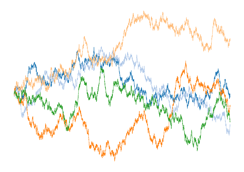
Figure 1: Plot of five different instantiations of the
discretized Wiener process generated using the code above.
Geometric Brownian Motion
With the Wiener process in hand, we can next explore a slightly more complicated
stochastic processes named Geometric Brownian motion (GBM). Like a Wiener
process, GBM is a continuous time stochastic process. GBM, however, assumes
a logarithmic dependence on an underlying Wiener process with drift. The
equation for such a process is
\[dS_t = \mu S_t dt + \sigma S_t dW_t,\]
where $S_t$ provides the time index for the value of the stochastic process,
$\mu$ is the constant related to the drift, $\sigma$ represents the volatility
of the process, and $W_t$ is the Weiner process. This model is simple enough to
be solved analytically, with the solution being:
\[S_t = S_0 e^{\left(\mu - \frac{\sigma^2}{2}\right) t + \sigma W_t}\]
but this does not limit the applicability of GBM. In fact, GBM has seen
applications in a wide range of fields including finance through the
celebrated Black-Scholes model and other financial models, molecular dynamics,
and even genetics. GBM is popular in all of these areas because it is
intuitively easy to grasp, and easy to modify to include new physics such as
stochastic jumps or non-constant volatility.
While an analytic solution is useful, we will compute trajectories of the GBM
by discritizing it on a grid, and using the cumulative summation that we used
above for the Wiener process. In code, this looks like:
import numpy as np

def GBM(N=10000, mu=1.0, sigma=0.8, s0 = 1.0):
    t = np.linspace(0.,1.,N+1)
    dt = 1./N
    dW = np.random.normal(0., 1., int(N + 1)) * np.sqrt(dt)
    W = np.cumsum(dW)
    term1 = (mu - sigma**2/2.0) * t
    term2 = sigma * W
    S = s0 * np.exp(term1 + term2)
    return t, W, S
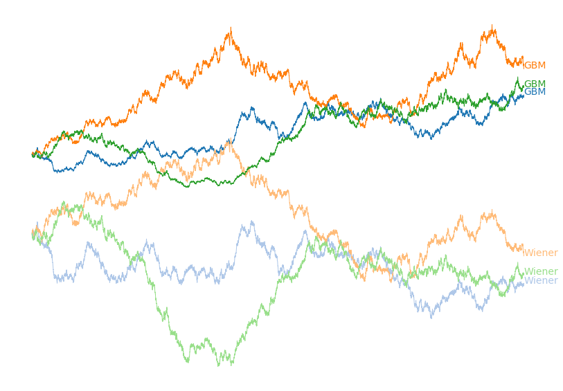
Figure 2: Plot of three different instantiations of the
discretized Geometric Brownian motion process and the underlying Wiener process
generated using the code above. Matching colours have the same underlying
stochastic processes.
To model real world data with a GBM we can compute the drift and volatility from
the data at hand, and then project forward many trajectories to understand
the likelihood of many future possibilities.
Building a model of Cash on Hand
With an understanding of some stochastic processes in hand, we next seek to
actually model personal financial data. One of the most important values to
track when evaluating financial health is cash on hand. Obviously you generally
want to spend less than your income, but how much less? And what are the
effects of activities like buying a house, increasing rent, raises, having
kids, vacations, and other life events on cash on hand?
The most straight forward starting point is to model personal spending habits.
Having analyzed my last 6 years of spending, they been constant with minor
fluctuations once major life events such as paying for a wedding were
subtracted. There also rarely appears to be any obvious memory from month to
month. Because I mostly observed fluctuation of a calculable standard
deviation around a calculable mean, with no historical dependence, we seem to
meet most of the conditions for Wiener process model to hold.
To build out this model, let’s assume an after-tax salary of $1000/month and a
year of spending data that looks like the following:
[ $1106.95 $819.1 $782.45 $629.3 $951.48 $795.21 $955.4 $1004.88 $1109.47 $1277.65 $1380.51 $1058.21]
We can then compute the mean and standard deviations to arrive at data driven
values for our financial model. This can be simply done by:
mean = np.mean(spending) # $989.22
std = np.std(spending) # $206.37
We can then generate a single forward trajectory of cash on hand with these
values using the following code, which is closely related to the previous code:
N = 60 # 5 Years
dW = salary - np.random.normal(mean, std, int(N))
W = np.cumsum(dW)
where $W$ now represents our time dependent cash on hand. We can generate a
single trajectory, but this is hardly going to be a valuable exercise
because the odds of accurately predicting future cash on hand is extraordinarily
low. Instead, we can understand the result of the trajectories in distribution
by running many trajectories and exploring their distribution, which we have
plotted below in Figure 4:
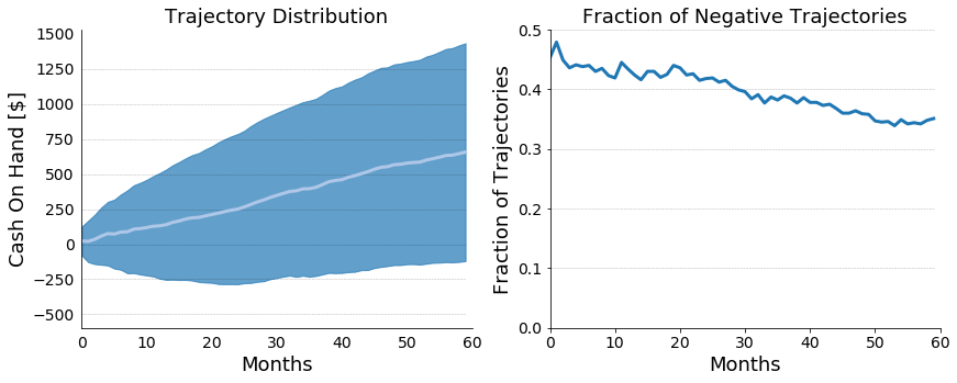
Figure 3: On the left, a plot of projected cash on hand for
our hypothetical financial scenario. The mean trajectory is plotted in white,
and the standard deviation is plotted in blue. On the right, a plot of the
fraction of trajectories with a negative cash on hand.
From simple subtraction, we knew that the hypothetical person in the above
scenario would be struggling, because, on average, there was only this person
could only expect to save $10.78/month. It’s safe to say that the above
scenario isn’t financially healthy, but we now have a firm sense for how
unhealthy this exact scenario is. With already an extremely simple model,
we can already start to appreciate the depth of questions that we can ask.
Beyond that, however, we can also start to appreciate the true randomness that
underpins life; which I’ve found to be useful in distressing budgeting for the
future in uncertain situations.
Adding Time Dependence
Let’s take this model and run with it! My spending habits tended to have natural
cyclic variation, with higher spending around Christmas time (presents and
plane tickets to visit family) and the summer due to vacations. The plan is to
make the mean for our Wiener process time dependent. For the sake of this
simulation, we will explore the financial situation around hypothetical person
2 (HP2), who we assume has a take-home salary of $3000/month, and we will assume
the following means for our stochastic spending process:
| Month |
Mean [$] |
Notes |
| Jan |
2000 |
|
| Feb |
2000 |
|
| Mar |
2000 |
|
| Apr |
2000 |
|
| May |
2000 |
|
| Jun |
4000 |
Vacation |
| Jul |
2000 |
|
| Aug |
2500 |
Back to School |
| Sep |
2000 |
|
| Oct |
2000 |
|
| Nov |
3500 |
Christmas Plans Booked |
| Dec |
3000 |
Christmas Gifts |
With a simple modification, we can just plug these values right in:
dW = []
salary = 3000
for i in range(N):
    monthly_spending = np.random.normal(SpendingMeans[i % 12], 300., 1)[0]
    dW.append(salary - monthly_spending)
W = np.cumsum(dW)
We can simulate just like before, and we can study distributions in the way
to understand our HP2’s potential envelope of futures. These distributions
are plotted in Figure 5:
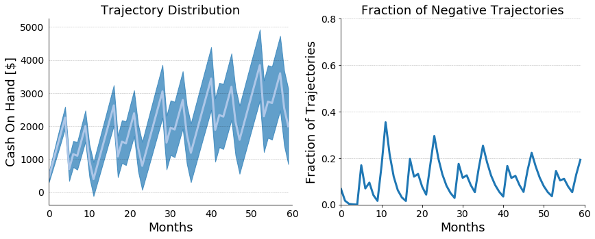
Figure 4: On the left, a plot of projected cash on hand for
our hypothetical financial scenario with time dependent means. The mean
trajectory is plotted in white, and the standard deviation is plotted in blue.
On the right, a plot of the fraction of trajectories with a negative cash on hand.
Modeling Salaries With Stochastic Jump Process
Up until now we’ve provided a somewhat coarse model for household spending but
we’ve ignored the general stochasticity of compensation that comes from raises
and bonuses. Over a multiyear projection, ignoring these compensation increases
can lead under-forecasting of cash on hand. For the sake of modeling, I’m going
to assume that our hypothetical person 2 (HP2) is a salaried individual, who
is making 3000/month after taxes and averages a 4% raise year over year with a
standard deviation of 2%. This volatility can come from market conditions,
HP2’s individual performance, or performance of his employer. Whatever the
case, capturing this variability will have a drastic impact on the accuracy of
our cash on hand simulations.
To do this we will start by assuming a yearly raise cycle, where the raise
amount is drawn from a normal distribution that is constrained to be positive.
mean_raise = 4.0 # Can be computed
std_raise = 1.0 # Can be computed
base_salary = 3000 # per year
p = 1.0 # Base percentage

salary = np.array([base_salary] * N)
for i in range(len(salary)):
    if (i != 0) and (i % 12) == 0:
        p = p * (1. + np.abs(np.random.normal(mean_raise, std_raise))/100)
    salary[i] = salary[i] * p
| Year |
Mean Yearly Salary |
| 0 |
29400.0 $\pm$ 0.0 |
| 1 |
30577.0 $\pm$ 293.61 |
| 2 |
31802.77 $\pm$ 431.88 |
| 3 |
33075.85 $\pm$ 551.76 |
| 4 |
34397.68 $\pm$ 662.16 |
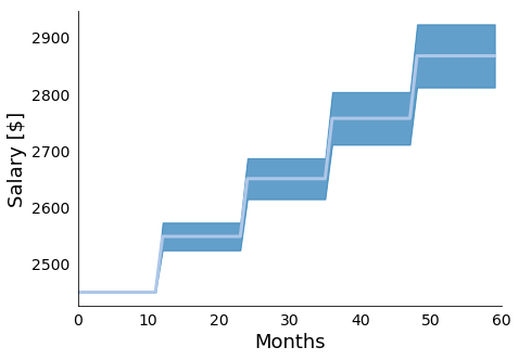
Figure 5: In Figure 5 we present the mean and standard
deviations of 10000 simulations of the presented yearly raise model. We see the
expected stair step pattern, with more uncertainty as we project further into
the future.
With this simple model in hand, we will next assume stochasticity with respect the
interval between raises. This distribution matches roughly the raise and
promotion cycle that we generally experience in our jobs. That is, generally
our raises correspond to yearly performance reviews, but promotions and raise
cycles can come a touch earlier or a touch later. We will build this
stochasticity in by drawing the periods between raises from a Poisson
distribution with rate $\lambda$ and a linear shift. To provide an intuition
for what the Poisson distribution looks like, I’ve plotted a histogram of
100000000 samples below in Figure 6.
def poisson_draw(lam = 2, shift = 0, truncate = False):
    while(1):
        val = shift + np.random.poisson(lam)
        if not truncate or (truncate and val >= 0):
            break
    return val
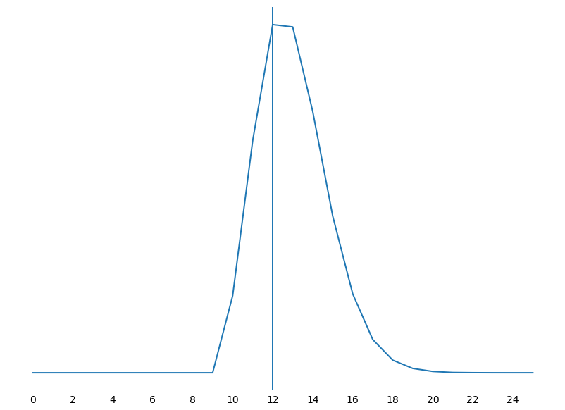
Figure 6: In Figure 6 we present the poisson histogram that
is generated by drawing 100000000 samples from the above function with lam = 3
and shift = 10. As expected, we see our most likely period as 12 months but we
have some statistical support around a slightly early raise or a delayed raise,
with the delay being more likely than the early raise.
With a duration model in hand, we can then modify our simple stochastic raise
model to include a stochastic time dependence between raises. This can be done
simply by drawing the raise period from a poisson distribution, as indicated
below:
last_raise = 0
raise_period = poisson_draw(lam = 4, shift = 8)
for i in range(len(salary)):
    if (i != 0) and (i  - last_raise) == raise_period:
        pp = np.abs(np.random.normal(mean_raise, std_raise))/100.
        p = p * (1. + pp)
        last_raise = i
        raise_period = poisson_draw(lam = 4, shift = 8)
    percentage.append(p)

for i in range(len(salary)):
    salary[i] = salary[i] * percentage[i]
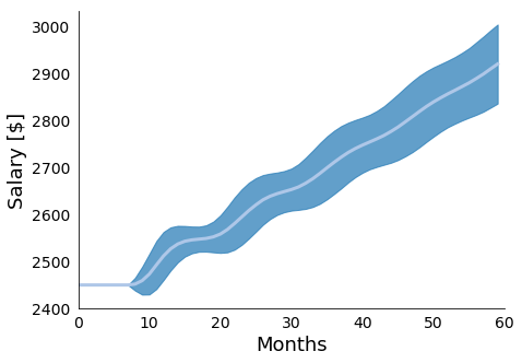
Figure 7: In Figure 7 we present the mean and standard
deviations of 10000 simulations of the presented raise model with stochastic
raise periods. We see the stair step pattern gets "smeared" out due to the added
uncertainty, with more uncertainty as we project further into the future.
| Year |
Mean Yearly Salary |
| 0 |
29475.97 $\pm$ 108.38 |
| 1 |
30614.07 $\pm$ 369.22 |
| 2 |
31825.85 $\pm$ 533.17 |
| 3 |
33093.98 $\pm$ 671.24 |
| 4 |
34416.07 $\pm$ 803.32 |
The second major source of randomness in HP2’s compensation is the role of
bonuses in total compensation. Bonuses typically fall within a range of
percentage of salary, and are typically offered at the end of the year, which
is how we will choose to model them in this case. Specifically, we will assume
that HP2 has a 5% yearly bonus optionality, and that HP2 is bonused every
December. This model is probably the simplest that we have to implement, and
the code looks something like:
def bonus_model(bonus_mean, bonus_std, yearly_salary):
    N = len(yearly_salary)
    bonus_percentages = np.random.normal(bonus_mean, bonus_std, N)/100.
    bonus = []
    time = []
    i = 0
    for j in range(12*N):
        time.append(j)
        if (((j % 12) == 11) and j != 0):
            bonus.append(bonus_percentages[i] * yearly_salary[i])
            i = i + 1
        else:
            bonus.append(0.0)
    time = np.array(time)
    bonus = np.array(bonus)
    return bonus, time
Putting It All Together
Because our observable is cash, we can combine all of these models with through
simple addition. This allows us to represent our total compensation model as:
salary, yearly_salary = stochastic_raise_salary_model(base_salary, mean_raise, std_raise, N)
bonus, months = bonus_model(mean_bonus, std_bonus, yearly_salary)
total_comp = (salary + bonus)
Putting this all together, we can combine the cyclic spending model with the
above total compensation model to arrive at a richer set of simulations, which
we present in figure 6.
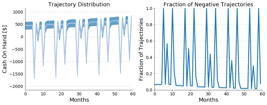
Figure 8: In Figure 8 we present the cash on hand model that
combines together the stochastic salary model with stochastic raise periods,
stochastic bonus model, and cyclic stochastic spending model. Taken together
we see that over the 5 year period our HP2 slowly becomes more financially
stable, but still caries significant debt year after the holidays every year.
Conclusions
These models were extremely simple but can be combined and extended with more
parameters to account for deterministic things such as event based tax benefits
(e.g. the interest deduction from buying a house), stock market performance,
credit card debt, and other important events. I’ve done precisely this and
they’ve already helped me to understand my finances more completely. Beyond
this, they’ve also helped to reduce my overall anxiety around finances because
uncertainty is a first class citizen of this approach.
Of course, beyond just extending these models, we also want to evaluate them
and then use real-world data to inform them so that we can plan using a true
posterior rather than just trying to draw inferences from our prior. I’ve chosen
to do this personally by likelihood weighting my trajectories. This is commonly
known as Approximate Bayesian Computation (ABC), and a followup post will detail
how I used ABC by implementing a very special purpose probabilistic programming
language.
[1] Please also note that any dollar figures quoted here are purely
hypothetical due to the highly private nature of personal finances. This does
not affect our modeling techniques, however.